Creating and Examining Spectra

While we believe there is great value in extracting info directly out of sightlines with clever use of binning, column densities, and ratios, some analysis can only be done with realistically generated spectra. This includes velocity analysis and component alignment analysis. So, here we include a number of tools for creating and easily plotting the results of spectra, as well as analysis tools to detect components.

Creating Spectra

To create a spectrum, you need start and end points. If you’ve generated points from quasarscan already (see Creating Sightlines), those will work fine, but any unitary points will work. This is a minimal script here. If you get a line with nothing in it (we’ll show how to display your line below), put the location of a galaxy for the ‘center’ in unitary length. By design, this creates a custom instrument with arbitrary resolution and which includes the line of interest in its redshift range – but depending on your code’s redshift, this might not align at all with COS or another real instrument!

import yt
from quasarscan.spectra.run_sightlines import run_line

sim_name = 'EXAMPLE'
sightline_num = 0
fname = '/loc/of/snapshot.hdf5'
ds = yt.load(fname)
center = ds.arr([0.5,0.5,0.5],'unitary')
start = center+ds.arr([0.05,0.05,0.05],'unitary')
end =   center-ds.arr([0.05,0.05,0.05],'unitary')
line_list = [('O VI', 1031.912)]

run_line(sim_name,sightline_num,ds,start,end,line_list)

The above code creates a series of files, one for each line given (so in this case, just one). It’s located in ~/spectra_from_trident/Ion_Spectra/EXAMPLE/<sim-exact-redshift>/Line_0/O/O VI_1031.912.txt. These folders are overkill for now, but they are very useful when you run many sightlines with multiple absorption lines in each one. What’s in that file is a set of wavelength[A], tau, flux, and flux_error, where the first and third columns are used as x-y coordinates for plotting spectra.

The list of arguments for run_line is shown here:

• sim_name: str The simulation name. This doesn’t interact with the name from other parts of quasarscan, this is just for categorizing the file it saves

• sightline_num: int This also just is used for categorizing the file (assuming you make multiple lines through it)

• ds: the (preloaded) yt Dataset

• start: list or array of three points, where to start the sightline. Trident takes points as unitary meaning all three dimensions should be between 0 and 1.

• end : list or array of three points. Same conditions as start

• lines: list of tuples, where the first element of each tuple is the ion name, and the second element is the rest wavelength of the transition. You can access these easily using the function quasarscan.spectra.trident_interfacer.get_line_list

• loc = 'default': str where to write spectra to. The names of the internal folders are hard-coded, but the location of the root directory can be specified here.

• metal_function = None: This can only be None or agora for now. If None, use trident default metals, if agora then use the agora-specific metal loading system (currently only available on my fork of trident)

• line_spec_width = 15: float how large to make the output file in angstroms, on either side of the rest-frame wavelength

• dlambda = 0.1: float The spectral resolution. I personally think idealized spectra are more useful for analysis, but you can make this coarser to be more like observations, or to be more memory efficient.

NOTE: running this in a cosmological simulation with default trident installed will cause some weird behavior. This is because trident by default redshifts the line relative to its length, with the line starting point at the redshift of the box, and then blueshifted with distance. This gives a bias towards negative velocities. In my personal fork of trident this code is replaced with the constant redshift of the box, meaning velocities will be more accurate (but many clouds far away from each other, like the Lyman alpha forest, will no longer work properly).

Interpreting Spectra

One important thing to do with spectra is identify absorption lines. The way this code is set up, there is no possibility of “line confusion” or anything like that, as each file is only a single line (within 15 or so angstroms). We use the Trident built-in fitter for the absorption lines to identify velocity components. This doesn’t perfectly identify the lines, but it does quite well. We also group together many aligned lines into “components” within 15 km/s of each other. The following code identifies lines:

from quasarscan.spectra.spectrum_analysis import load_file
from quasarscan.spectra.trident_interfacer import call_trident_fitter
from quasarscan.spectra.trident_interfacer import one_line_interpreter
from quasarscan.spectra.data_objects import alignment_checker

f_name = '~/spectra_from_trident/Ion_Spectra/EXAMPLE/<sim-exact-redshift>/Line_0/O/O VI_1031.912.txt'
wl,fl,redshift = load_file(f_name)
line = ('O VI', 1031.912)
fitted_lines, fitted_flux = call_trident_fitter(wl,fl,line = line)
checked_line = one_line_interpreter(wl, fl, fitted_lines, redshift, line, 0.95,bv_adjust = bv_adjust)
check_lines = [checked_line]
comps = alignment_checker(check_lines, 15)

The list of arguments for call_trident_fitter is shown here. This returns a dictionary of lines, containing their wavelength, b parameter, equivalent width, etc.:

• wavelength: array numpy array of wavelengths (returned by load_file)

• flux: array numpy array of fluxes at each wavelength (returned by load_file)

• trident_filename=``default``: str This uses the list of lines trident uses, stored inside your trident source code directory. If you installed trident at your home directory (either the base version or my fork), this should work fine.

• line = None: tuple where the first element is the ion name, and the second element is the rest wavelength of the transition. You can access these easily using the function quasarscan.spectra.trident_interfacer.get_line_list. If None, it will return empty dictionaries.

• maxNumComps = 8: int number of components to attempt fitting at once. Default is 8, as that is what trident does by default.

• kwargs: dict of other args for the call to trident.absorption_spectrum.absorption_spectrum_fit.generate_total_fit. See the trident documentation for details

A few of these features rely on using my fork of trident (such as being able to change maxNumComps), though this turns out not to matter very much for most purposes.

The list of arguments for one_line_interpreter is shown here. This takes that dictionary of lines and creates a list of AbsorptionLine objects, which can access some of the above values more easily (and do things like plotting itself):

• wl: array numpy array of wavelengths (returned by load_file)

• fl: array numpy array of fluxes at each wavelength (returned by load_file)

• fitted_lines: dict of lines returned by call_trident_fitter

• cosmo_redshift: float, the redshift of the simulation

• line: tuple, where the first element is the ion name, and the second element is the rest wavelength of the transition. You can access these easily using the function quasarscan.spectra.trident_interfacer.get_line_list

• fluxthreshold = 0.99: float, minimum value of flux before a line is “counted”

• bv_adjust = None: float velocity offset of the sightline relative to the bulk velocity of the halo in question in km/s. If None, just report physical velocities

• loud = False: bool if True, print the lines as they are made

alignment_checker takes in this list of AbsorptionLines, and returns a list of Components, each of which includes a list of all the lines within a certain velocity of one another.

Plotting Spectra

Now that we’ve found the lines in our spectra, we can pretty easily plot the data. It’s generally most useful to plot them in velocity space, because as we said it is most useful to check alignments between lines, rather than just getting column densities, which in a simulation we can extract much more straightforwardly. However, both velocity space and wavelength space plots are available.

from quasarscan.spectra.spectrum_analysis import load_file,plot_vel_around_line
import matplotlib.pyplot as plt

f_name1 = '~/spectra_from_trident/Ion_Spectra/EXAMPLE/<sim-exact-redshift>/Line_0/O/O VI_1031.912.txt'
wl,fl,redshift = load_file(f_name)
line = ('O VI', 1031.912)
ax = plot_vel_around_line(wl,fl,line,redshift,left_distance = 200)
#if you've saved some lines and components
for l in check_lines:
    l.plot_data(ax)
for c in comps:
    c.plot_data(ax)

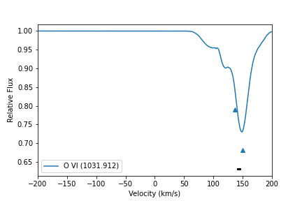
Here the actual spectrum is plotted in blue, and the detected lines as blue triangles. Components (which, generally, would contain multiple lines) are a black bar plotted below all the detected line indicators.

The list of arguments for plot_vel_around_line is shown here.

• wl: array numpy array of wavelengths (returned by load_file)

• fl: array numpy array of fluxes at each wavelength (returned by load_file)

• line = None: tuple where the first element is the ion name, and the second element is the rest wavelength of the transition. You can access these easily using the function quasarscan.spectra.trident_interfacer.get_line_list. If None, it will return empty dictionaries.

• cosmo_redshift: float, the redshift of the simulation

• noise = 0: float, standard deviation of a noise vector. Because fluxes are normalized, this is 1/SNR if you prefer to use a signal-to-noise ratio.

• color = ‘default’: matplotlib color variable. If default, then look up if this line has a default color, otherwise use matplotlib defaults

• left_distance = 200: float velocity to extend to on left of rest velocity

• right_distance = default: float velocity to extend to on right of rest velocity. By default, use same as left_distance.

• label = ‘default’: str label to send to matplotlib for legend (but you will have to call legend yourself)

• ax = None: matplotlib.Axis. The axis on which to plot the data. If None, make a new axis (return it at end)

• plot_chunk = ‘lims’: 'lims', 'all', or float. If lims, plot only data within the distances that will be shown. If all, plot all the data, even though it would not be shown. If float, plot only within plot_chunk in velocity space of the center, regardless of what will be shown

• bv_adjust = None: float velocity offset, will be added to the x axis.